
Introduction
In a context where the supply chain has become a central and structuring component of the Industry 5.0 ecosystem, recent research is shifting toward a new paradigm: Supply Chain 5.0. This paradigm aims to integrate advanced technologies in order to design highly intelligent, adaptive, and sustainable logistics networks.
Among the key topics associated with Supply Chain 5.0, inventory management plays a central role. In particular, the stock size problem, which consists of determining the optimal inventory levels to maintain for each spare part, especially in the context of preventive maintenance operations.
This problem is particularly critical as it arises in real-world environments characterized by a high level of uncertainty, such as demand fluctuations and unexpected supply disruptions. In this context, effective inventory management becomes a key lever to:
- improve the overall performance of the supply chain,
- maximize stakeholder satisfaction,
- minimize total costs (e.g., holding costs and shortage costs).
However, this work initially focuses on the static version of the stock size problem, without considering uncertainty.
Stock Size Problem definition
According to the initial definition proposed by Kellerer et al. (1998), the static version of the Stock Size Problem (SSP) considers a set of tasks to be executed over a given time horizon. Each task either consumes or generates a certain amount of resources, thereby impacting the inventory level. From an Operations Research perspective, the SSP is generally formulated as a multi-SKU inventory optimization problem under capacity constraints.
In an industrial context, the problem can be stated as follows: determine the required storage capacity and its optimal allocation, across different products and locations under given constraints. In maintenance applications, these products correspond to spare parts required for preventive maintenance operations. The problem therefore consists of allocating a limited storage capacity among multiple spare parts and across different levels of the supply chain, while ensuring a desired service level and minimizing costs. The key decisions involved include determining the maximum storage capacity, selecting the number of items to be stocked, and allocating inventory among suppliers, warehouses, and consumption sites.
In more realistic industrial environments, the SSP extends to dynamic and stochastic settings, incorporating demand uncertainty and temporal evolution. It is therefore embedded within multi-period planning frameworks, where inventory levels evolve over time and decisions are made at each period, including replenishment, inventory carryover, and the management of demand variability.
Overall, the Stock Size Problem provides a fundamental basis for modeling inventory management systems, evolving from a simplified static framework to more realistic dynamic and stochastic approaches aligned with industrial practices.
Study context and assumptions
Based on the Work Order (WO) historical data, we perform a static optimization to determine the stock size of each item in order to satisfy the overall demand over a given horizon.
The objective of the basic model is to determine, for each item:
- the initial stock quantity,
- the on-hand inventory at the end of each day t within the horizon,
- the backorder quantity at the end of each day t within the horizon,
while minimizing the total cost, defined as:
Total Cost = Purchase Cost + Holding Cost + Backorder Penalty Cost.
For the experiments, the dataset used is an open dataset available at Comprehensive Supply Chain Analysis . This dataset contains historical regional sales data from the United States, providing detailed transactional information across multiple sales channels. Although it is originally sales-oriented, we assume that each “product” corresponds to an “item” required for a maintenance intervention. In this context, price-related information is ignored and the analysis focuses on quantities, which constitute the primary variables of interest.
Assumptions
- No replenishment is considered. For example, when backorders occur, a penalty is applied.
- The holding cost and backorder penalty are determined using two parameterizable rates. These costs are computed based on the average purchase cost of the product.
- No variability is considered in this model. The demand for each item on day t within the planning horizon is assumed to be known in advance, as provided in the dataset.
- No constraints (such as service level or safety stock constraints for each item) are included in this basic model. Note that this model serves as a foundation to ensure a clear understanding of the target problem.
Prototype architecture overview
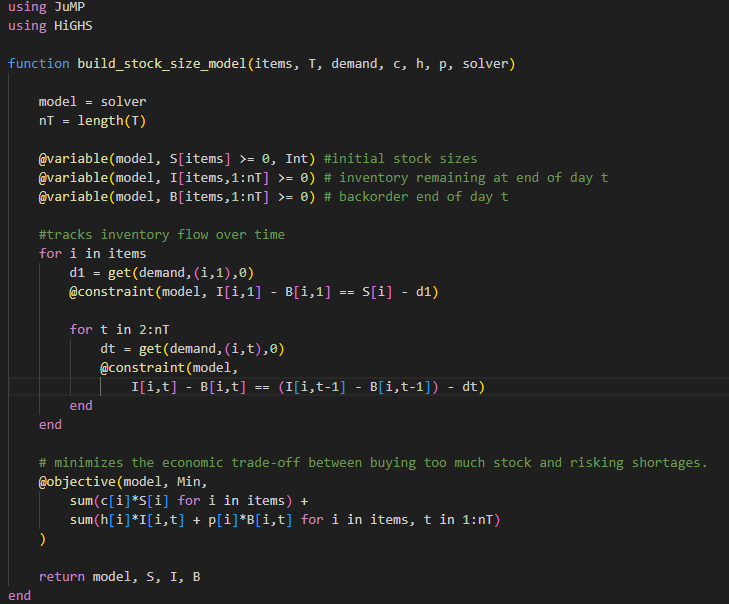
Integer Linear Programming (ILP) Model description
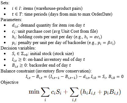
A brief explanation of the objective function
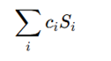
This refers to the purchase cost, meaning the cost incurred when buying the initial stock. The greater the inventory level, the higher the total purchase cost.
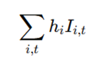
This refers to holding costs, the costs associated with maintaining inventory in stock, including warehousing, capital, and storage costs. The higher the inventory level, the higher the overall holding costs.
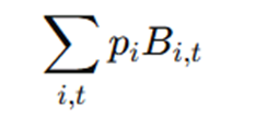
This refers to the backorder penalty cost, which arises when demand cannot be fulfilled because of insufficient inventory. Such situations may lead to customer loss, reduced service levels, and the payment of penalty costs.
Architecture description, why JuMP ?
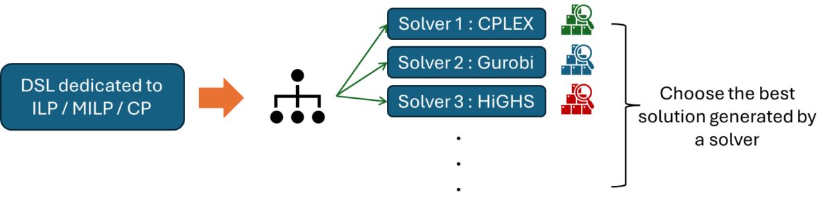
Frequently, we encounter difficulties when experimenting to evaluate the optimization results of our model or when developing alternative solutions. This can be time-consuming, as it often requires learning and using another Domain Specific Language (DSL) to build a different model.
In this study, we adopt an existing and popular DSL dedicated to ILP / Mixed-Integer Linear Programming (MILP) / Constraint Programming (CP). The model written using this DSL is compatible with a series of state-of-the-art commercial or free-to-use solvers for solution generation. This allows us to easily conduct comparative studies on solution quality without significant additional effort.
Several DSLs are available on the market (open-source) for developing ILP/MILP/CP models, notably Pyomo, JuMP, and PuLP. As a first step, we conducted a comparative analysis of these three DSLs.
| Tool | Language | Best For | Nonlinear | CP | Performance | Commercial-ready |
| PuLP | Python | Small/medium LP/MILP | No | No | Medium | Yes |
| Pyomo | Python | LP/MILP/NLP/MINLP | Yes | (not native CP) | Medium | Yes |
| JuMP | Julia | Large-scale, high-performance optimization | Yes | Via solver | High | Yes |
After this initial summary analysis, we can conclude the following:
- If performance is the main concern : JuMP
- If staying within Python is required : Pyomo
- If only simple MILP problems need to be solved : PuLP
Since we do not have constraints regarding the programming language, and we are not limited to solving only MILP problems in our modeling, performance is essential for us, especially when addressing industrial-scale use cases. Therefore, JuMP, based on Julia, is the most suitable choice.
Then, a series of comparisons further supports our choice:
Compatibility of the DSL with the solver ecosystem
| Solver | Type | Works With |
| CBC | MILP | PuLP, Pyomo, JuMP |
| HiGHS | LP/MILP | Pyomo, JuMP |
| GLPK | LP/MILP | All |
| SCIP | MILP/MINLP | Pyomo, JuMP |
| IPOPT | NLP | Pyomo, JuMP |
| Bonmin | MINLP | Pyomo, JuMP |
| Couenne | Global MINLP | Pyomo, JuMP |
| OR-Tools CP-SAT | CP/MILP | Python direct (not PuLP/Pyomo native) |
Performance Comparison
Model Construction Speed : JuMP > Pyomo > PuLP
JuMP is extremely fast because:
- Julia is compiled
- Uses efficient MathOptInterface
- Avoids Python overhead
For very hard problems (MILP/ILP), the following strategies can be applied:
- Use solver heuristics
- Use time limits
- Enable MIP gap (e.g., 5%)
- Use relaxations
All three DSLs (PuLP, JuMP, and Pyomo) support these features through solver parameters.
Prototype architecture
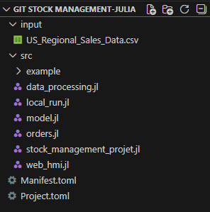
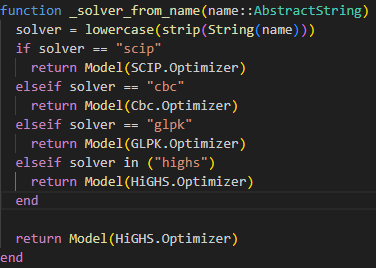
For more details, we present below the model view and the solver integration view. We have integrated 4 high-performance, free-to-use solvers from the list of compatible solvers.
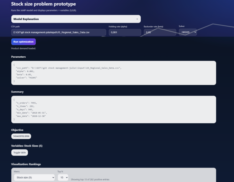
Finally, we provide an overview of the web UI of our prototype. The figure illustrates a web-based prototype for solving the Stock Size Problem using a JuMP-based optimization model. The interface enables the configuration of key parameters, including the dataset path, the holding cost ratio (α), and the backorder cost ratio (β), both defined relative to the unit cost of each item, as well as the choice of solver.
Once the optimization is executed, the system provides summary statistics of the dataset and reports the resulting objective value. The optimized stock levels for each item are computed and can be explored through a ranking-based visualization, highlighting the most significant inventory allocations.
Conclusions
This work represents an initial step in our research on stock management within the context of Industry 5.0. Through an accessible prototype, we illustrate the Stock Size Problem, which constitutes a fundamental problem in inventory management in this domain.
The use of JuMP as a modeling framework provides significant flexibility by enabling seamless integration with multiple state-of-the-art solvers, thereby facilitating comparative analysis and improving solution robustness. More broadly, this work demonstrates how such approaches can help bridge the gap between theoretical developments in Operations Research, and real-world industrial decision-making support.
As future work, we aim to extend this research by integrating business-oriented constraints tailored to different clients in a generic and scalable manner. Furthermore, incorporating real-world dynamics, including uncertainty and stochastic events, will constitute a key challenge to address.
References
Kellerer, H., Kotov, V., Rendl, F., Woeginger, G.J.: The Stock Size Problem. Oper. Res. 46, S1–S12 (1998). The Stock Size Problem | Operations Research .