As you know at Berger-Levrault, we are not afraid of challenges, on the contrary, we take them up with pleasure!
Asset Performance 4.0 is a virtual conference and exhibition to learn how new 4.0 technologies and the fundamentals of operations, maintenance and asset management reinforce each other to improve equipment reliability and cost performance in asset-intensive industries. This virtual conference and exhibition will take place from 15 to 17 September 2020.
Before the conference, Asset Performance 4.0 has organized 3 Hackathons on recent maintenance topics.
CARL Software participated in one of the Hackathons, the topic of which is :
“Fluvius: predicting failures based on sensor and humidity data.“
Following its presentation, CARL Software was one of the finalists in the challenge.
The Context
1. Current system:
Currently, electrical substations are equipped with humidity and temperature sensors. Condensation (the result of high humidity and low temperature) can shorten the life of electrical equipment, so it is necessary to detect failures in the heating system and water in the basements.
Today this detection is done by a fixed threshold on temperature and humidity. This threshold can be adjusted manually and therefore there is no intelligent system that would use historical or contextual data to improve the threshold.
However, the system is prone to high rates of false alarms, which means that there are many alerts and eventually real damage, which tends to make us ignore them. But, reducing thresholds to lower the alerts can result in missing failures.
In conclusion, in both cases, the alert system becomes obsolete.
2.The desired improvements
The main objective of the project is to improve the warning system. It is strongly suggested to do so by defining more intelligent thresholds based on historical data (previous observations) and/or contextual data (weather, type of building, etc.). False alarms must be avoided, or at least detected to cancel the alert. The desired delivery is not a complete solution but a list of data processing steps to make the threshold more intelligent.
We were able to detect different types of phenomena on the data, depending on the sensor. Following the analyses, we were able to think about suggestions.
Our approach
- Timeseries forecasting to raise alarms:
Thanks to the implementation of ARIMA models, we can forecast the next values using those of the European Union.
This allows us to detect failures in the heating system.
However, this method is to changes the distribution of data.
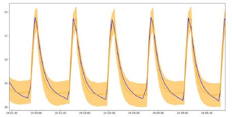
Predictions for the same distribution as the one the model was learned on 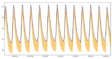
Predictions for a different distribution (higher values)
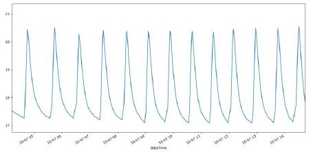
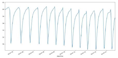
- Level the data by subtracting the rolling mean:
To avoid the problem mentioned above, we can subtract their moving average from the time series.
This is simple, but this proposal may lack precision where the changes occur.
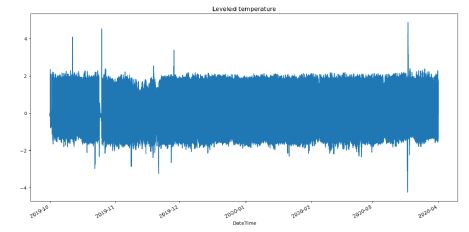
Levelled dataset, there is no more visible changes in amplitude 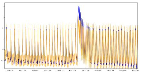
Prediction at a previously point of change
- Adapt the model with change detection:
A more sophisticated way to address the mentioned issue is to detect abrupt changes in the distribution and train a new model each time a change occurs. It avoids raising false alarms when
the changes occur, but it is possible that failures previously detected become invisible. The use of the different methods altogether is hence necessary.
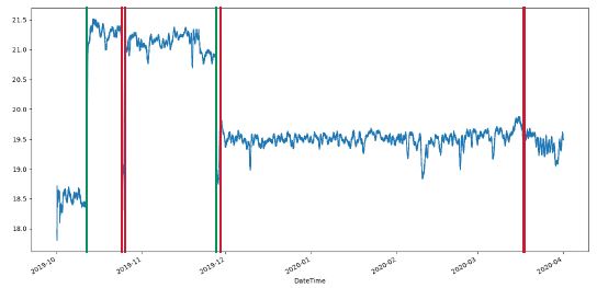
and expected but unwanted results (red)
- Improve the thresholds with rolling mean:
Because we can now detect the failures, the thresholds can be adapted with the use of the rolling mean as base. Far less alarms will be raised this way.
- Detect sensor failures with multivariate analysis:
We want to use the correlations between the variables to detect faulty sensors. Indeed, when a sensor generates incorrect values, this can trigger false alarms. However, if only one variable is affected, it means that the sensor is probably faulty, and we can avoid triggering an alert for failure.
Outcome of this Challenge
We have chosen to respond to this challenge with a list of suggestions, but we have focused primarily on the use of ARIMA models to correctly predict the given time series. However, our experience has allowed us to suggest other possibilities to be explored in order to improve the warning system.
In our opinion, the various suggestions made should be used together and adapted to each station. The objective is for users to receive alarms from different sources with the possibility of :
- Deactivate those that are not useful,
- Give priority to the most interesting ones,
- Cross them to generate new ones (for example ALARM_3 = ALARM_1 AND ALARM_2 or ALARM_6 = ALARM_4 NOR (ALARM_5 AND ALARM_3)),
- Adjust the parameters of their thresholds according to the confidence in the other alarms.
It would also be possible to develop a data visualization allowing users to play with the data and solutions to experiment with them in a playground.
For the suggestion regarding the current analysis strategy, we do not see the need to modify the current daily reporting system.
However, it would be more practical to have the same sampling strategy (in other words, the same period between measurements) for all sensors to make better use of the correlated variables.
Annexes
ARIMA and SARIMA models are adaptations of ARMA models. The objectives of these last ones are to make time-series forecasting (predict future observe with the sole knowledge of past observations). It is close to linear regression with the use of past data as predictors.
An ARMA model is composed of two parts. The first one is its AR (Auto-Regressive) component, which definite relation between an observation at the current time and the ones at previous times. The second one is its MA (Moving Average) component, which definite relation between an observation at the current time and the residual errors from the current and some previous timesteps. It is important to note that, theoretically, a process must be stationary to be able to be strictly described by an ARMA model.
However, the stationarity of the process is difficult to obtain because time-series have non-stationary components (trend and seasonality). It still exists in ways to transform the process until stationarity can be accepted.
The first one is to differentiate the time series to remove the trend. The first order of differentiating apply the operator 1−𝐿 to the process, the second-order the operator(1−𝐿)2and the
𝑑-th order the operator (1−𝐿)𝑑, with 𝐿 the operator defined by 𝐿(𝑋𝑡)=𝑋𝑡−1 ((1−𝐿)(𝑋𝑡)=𝑋𝑡–𝑋𝑡−1). If 𝑌𝑡=(1−𝐿)𝑑(𝑋𝑡) is an 𝐴𝑅𝑀𝐴(𝑝,𝑞) process, then 𝑋𝑡 is an 𝐴𝑅𝐼𝑀𝐴(𝑝, 𝑑, 𝑞) process.
The second one is to also take the seasonality into account with a 𝑆𝐴𝑅𝐼𝑀𝐴(𝑝, 𝑑, 𝑞)×(𝑃, 𝐷, 𝑄)𝑠 process where the extracted process of the 𝑌𝑡=𝑋𝑖+𝑠*𝑡, 𝑖∈⟦0, 𝑠−1⟧ is an 𝐴𝑅𝐼𝑀𝐴(𝑃,𝐷,𝑄) process.
Explanation of SARIMA processes:
https://www.youtube.com/watch?v=YIoBRDueHKo
Even if it is written for Python users, the following guide is useful to understand how to parameterize an ARIMA model:
https://www.machinelearningplus.com/time-series/arima-model-time-series-forecasting-python/
For more details, do not hesitate to read the article below:
Hackaton-Fluvius-2020