SemEval is a series of international Natural Language Processing (NLP) research workshops whose mission is to advance the current state of the art in semantic analysis and to help create high-quality annotated datasets in a range of increasingly challenging problems in natural language semantics. Each year’s workshop features a collection of shared tasks in which computational semantic analysis systems designed by different teams are presented and compared.
In this edition, SemEval proposed 12 tasks to work on.
As you might know, NLP is a subject our team is dedicated to. SemEval was a great opportunity to challenge ourselves with an international NLP community. In this article, we’ll develop how our team members dealt with this first reverse dictionary task they chose: CODWOE: COmparing Dictionaries and WOrd Embeddings, which consists in comparing two types of semantic descriptions: dictionary glosses and word embedding representations. Basically, given a definition, can we generate the embedding vector of the target word?
Recent research focused on learning arbitrary-length phrases and sentences representations and the reverse dictionary is one of the most common cases to solve this problem. The reverse dictionary is the task to find the searched word through its description. For instance, by giving this description: “a piece of writing on a particular subject in a newspaper or magazine, or on the internet” to the reverse dictionary, it should find the word “article” corresponding to it.
The main problematic remaining is how to capture relationships among multiple words and phrases in a single vector?
The organization provided a trial dataset of 200 elements composed of definition and their embeddings vectors in five languages: French, English, Spanish, Italian and Russian and in different vectors representations built with well-known techniques:
- “char” corresponds to character-based embedding, computed using an auto-encoder on the spelling of a word.
- “sgns” corresponds to Skip-Gram with negative sampling embedding, aka. Word2Vec (Mikolov et al., 2013).
- “electra” corresponds to Transformer-based contextualized embedding.
In order to keep results comparable and linguistically significant, challengers were not able to use any external resources.
In the following, we’ll present our contributions to solve the reverse dictionary problem.
Our models proposition
Our approaches require a model able of learning to map between arbitrary length phrases and fixed length continuous valued word vectors. We explored sequential models, especially LSTM (Long-Short Term Memory) and BiLSTM (Bidirectional Long-Short Term Memory) models. Following models architecture are based on TensorFlow and Keras libraries.
Before introducing our models, we want to mention that we preprocessed the content data using Stanza which lemmatized all definitions and remove all the punctuation. We did it in order to minimize alternative words for a same concept and help our models to correctly process the vocabulary.
Baseline Model
Our first model called Baseline Model in intentionally simple to create baseline scores and introduce manipulations on the datasets.
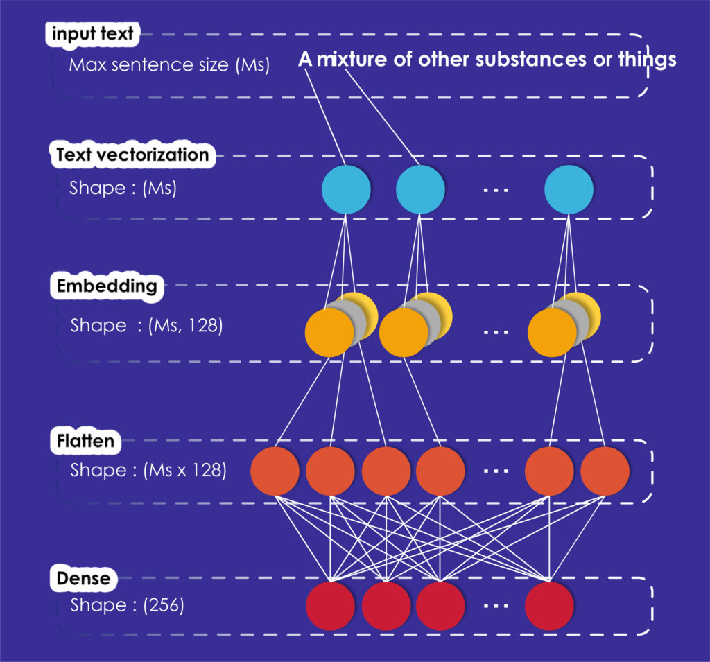
As you can see in figure 1, our model created with Keras is composed of four layers. Its first layer which is the text vectorization, transforms the input text in a vector. To perform this operation, we must give an identifier to each different word in our corpus, then each sentence will be represented as a vector of identifiers.
Now, each vector’s sentence is ready to be processed by the embedding layer which turns positive integers (indexes) into dense vectors of fixed size.
Then, the flatten layer will change the data dimension from two dimensions to one without losing any value.
Finally, we model the output data by using a fully connected layer (Dense layer) to match the gloss embedding given by the organizers.
Advanced Model
LSTMs are a Reccurent Neural Networks (RNN) which have an internal memory that allows them to store the information learned during training. They are frequently used in the reverse dictionary task and in word and sentence embedding tasks, as they can learn long-term dependencies between existing words in the sentence and thus compute context representation vectors for each word.
BiLSTM is a variant of LSTMs. It allows a bidirectional representation of words.
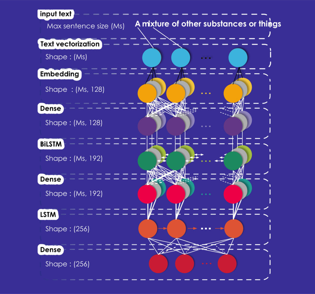
Our second model, named Advanced Model is a BiLSTM-LSTM network. As for the Baseline Model, we use a sequential model which can be provided by Keras.
This model also starts with a text vectorization layer, an embedding layer and a dense layer producing vectors. Then we added a BiLSTM layer, which takes a recurrent layer (the first LSTM of our network) which in turn takes the “merge mode” as an argument. This mode specifies how the forward and reverse outputs should be combined; in our case, the average of the outputs is taken.
To these three layers, we added another fully connected Dense layer and an LSTM layer of 256 dimensions corresponding to the dimensions of the output vectors and a final Dense layer with the same dimensions.
Experimental Setup
Since there were three types of vector representations proposed to us in this shared task, we used the same architectures to produce the three types of vectors. However, the data format given to input to the model is not the same for the three types. For the “electra” and “sgns” representation types, we prepared a vocabulary containing the words of the glosses of the “training dataset”, the words of this vocabulary were obtained by following the preprocessing step.
For the “char” vector type, we construct a vocabulary of all the characters used in the glosses without preprocessing the data. The idea being that, for the “char” type representation, the model encodes the glosses characters into vectors and then produce the vectors glosses encoding based on vectors of characters constituting the glosses.
The model we propose is a monolingual model (we trained it separately on the training dataset of each language). However, in order to evaluate the impact of using a multilingual model, we trained the same neural networks on five languages (with character vector) at the same time and compared the results obtained with those obtained by the monolingual models.
For the “sgns” and “electra” representation types, we built a vocabulary containing the words of all glosses on the five languages, which contains in total 121,147 words. We did the same with the “char” vectors but with preparing a vocabulary of characters instead containing 405 characters, in total. The table 1 below describes the vocabulary size for each monolingual model and for the multilingual model.
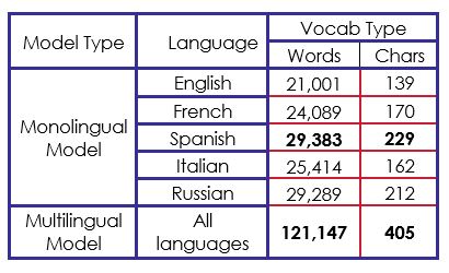
We notice that by adding all words in the five different languages of the original data, there are 129,176 words. Though our multilingual model vocabulary results of 121,147 words which means there are 8,029 common words between at least two different languages.
Results and Analysis
Our main goal was to outperform the organizer’s baseline model and results.
Our Baseline Model didn’t perform better than the state-of-the-art models, though, we can analyse an interesting point: this simple model surprisingly produces better results on the Rank cosine measure. On the results of the MSE (Mean Squared Error) measure, only three cases outperform the organizers’ baseline model. Moreover, every rank cosine measure is better.
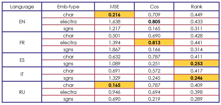
At this point, we can analyse that it’s hard to perform in the MSE and Cosine measures, while trying to get good results in the Rank measure and vice-versa. This analyse is supported by the following evaluation of our Advanced Model in table 3.
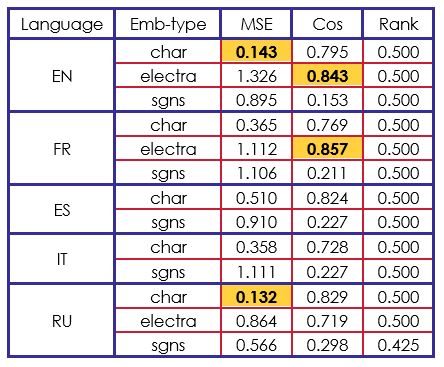
The results of our second model are completely opposite. We performed better than the organizer’s model in MSE and Cosine measures. On the other hand, the Rank cosine seems to be stuck at.
If we compare our results to other participants results, we can say that our BiLSTM-LSTM architecture is efficient on “char” and “electra” embeddings. For instance, in “char” with English, French and Spanish, we got the second-best score of the challenge.
Given the set of results obtained, we find that the best cosine score was obtained by using electra (contextualized) vector embeddings and the best MSE score was obtained by using character vector embeddings. More generally, the use of BiLSTM-LSTM architecture neural network has been beneficial in having results that surpass baselines when cosine and MSE are used as evaluation measures.
To conclude
In this article, we presented our contributions to solve the task 1 problem of the SemEval-2022 challenge. We studied the effects of training sentence embeddings with supervised data by testing our models on five different languages. We showed that models learned with char embeddings or contextualized embeddings can perform better than models learned with Skip-Gram word embeddings. By exploring various architectures, we showed that the combination of Embedding/Dense/BiLSTM/Dense/LSTM layers can be beneficial than the simple use of Embedding layer.
In a next article we’ll present our system for document-level semantic textual similarity evaluation at SemEval-2022 task 8: “Multilingual News Article Similarity”.
